STRINGutils Vignette
Chia Sin Liew
July 22 2021
STRINGutils_Vignette.RmdIntroduction
STRINGdb R package provides a convenient way to access the popular STRING database (https://string-db.org) from R. STRINGutils is built on top of STRINGdb and provides convenient functions to get SVG file of STRING network and highlight features of interest.
To prepare data necessary for STRINGutils, we first run code from STRINGdb vignette.
Briefly, we map the analyzed data of a microarray study to a human STRING database to get STRING identifiers. Please see STRINGdb vignette for more information.
string_db <- STRINGdb$new(version = "11", species = 9606,
                          score_threshold = 200,
                          input_directory = "")

data("diff_exp_example1")

example1_mapped <- string_db$map(diff_exp_example1, "gene", removeUnmappedRows = TRUE)
#> Warning:  we couldn't map to STRING 15% of your identifiers

hits <- example1_mapped$STRING_id[1:200]
Get SVG of STRING network
Once we have string_db, an instantiated STRINGdb reference class with associated information from STRING database, we can run the get SVG function. If file is specified, the SVG will be saved.
xml <- get_svg(string_db, hits)
xml <- get_svg(string_db, hits, file = "my_network.svg")Get full or subnetwork for proteins of interest
If we have a list of proteins of interest, the full or sub- STRING network of the proteins can be obtained. These proteins will be highlighted by the colors of choice.
For illustration purposes, here we will pick the top 10 proteins.
hits_filt <- example1_mapped %>%
  dplyr::slice_min(pvalue, n = 10, with_ties = FALSE) %>%
  dplyr::filter(!is.na(STRING_id)) # <- filter out proteins with no mapped STRING IDs
Let’s take a look at the proteins of interest. It is good to know that none of the top 10 proteins are missing STRING IDs.
| gene | pvalue | logFC | STRING_id |
|---|---|---|---|
| VSTM2L | 0.0001018 | 3.333461 | 9606.ENSP00000362560 |
| TBC1D2 | 0.0001392 | 3.822383 | 9606.ENSP00000481721 |
| LENG9 | 0.0001720 | 3.306056 | 9606.ENSP00000479355 |
| TMEM27 | 0.0001739 | 3.024605 | 9606.ENSP00000369699 |
| TSPAN1 | 0.0002393 | 3.082052 | 9606.ENSP00000361072 |
| TNNC1 | 0.0002921 | 2.932060 | 9606.ENSP00000232975 |
| MGAM | 0.0003051 | 2.369738 | 9606.ENSP00000447378 |
| TRIM22 | 0.0003235 | 2.293125 | 9606.ENSP00000369299 |
| KLK11 | 0.0003540 | 3.266867 | 9606.ENSP00000473047 |
| TYROBP | 0.0003593 | 2.410288 | 9606.ENSP00000262629 |
Next, we need to make a color vector of the same length as our proteins of interest to specify what colors to highlight our proteins with.
Let’s take a look at the color vector.
colors_vec
#>            VSTM2L            TBC1D2             LENG9            TMEM27
#> "rgb(101,226,11)" "rgb(101,226,11)" "rgb(101,226,11)" "rgb(101,226,11)"
#>            TSPAN1             TNNC1              MGAM            TRIM22
#> "rgb(101,226,11)" "rgb(101,226,11)" "rgb(101,226,11)" "rgb(101,226,11)"
#>             KLK11            TYROBP
#> "rgb(101,226,11)" "rgb(101,226,11)"Note: It is important to double check to make sure that the proteins of interest are matched up to their intended colors.
Now, we can go ahead and get the network. The function saves the network as a SVG file in the current directory as “features_of_int.svg”.
For full network:
plot_features(example1_mapped, colors_vec, string_db, entire = TRUE)
#> Getting 200 nodes from STRING network...
#> Table of features of interest is printed to: "table_features_of_int.csv"
#> NULL
The SVG file can be viewed with the magick::image_read_svg() function in RStudio viewer.
magick::image_read_svg("features_of_int.svg")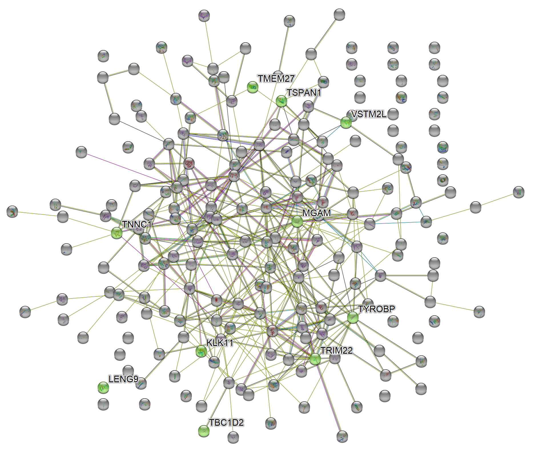
Full network
The default number of proteins obtained from the network is set to 200. This number can be changed with n_hits. The network view mode for STRING network can also be defined with network_flavor. More information about this can be found at STRING’s website.
For example, to increase the number of proteins in the network to 500 and use the network view mode of confidence instead of the default evidence:
plot_features(example1_mapped, colors_vec, string_db, n_hits = 500, entire = TRUE,
              network_flavor = "confidence")
#> Getting 500 nodes from STRING network...
#> Table of features of interest is printed to: "table_features_of_int.csv"
#> NULL
magick::image_read_svg("features_of_int.svg")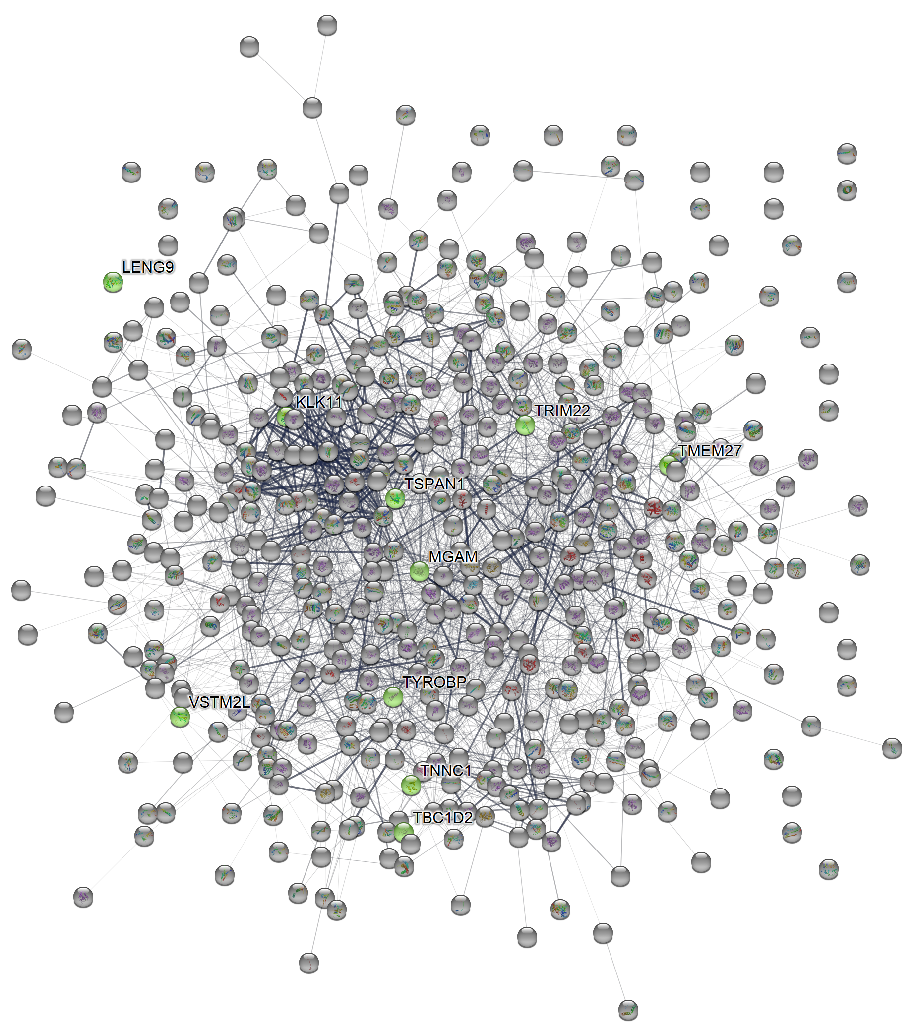
Full network, higher n_hits
For subnetwork:
plot_features(example1_mapped, colors_vec, string_db)
#> Getting 200 nodes from STRING network...
#> Table of features of interest is printed to: "table_features_of_int.csv"
#> --------------------------
#> Cluster 2 is a hit
#> 9606.ENSP00000232975 | 9606.ENSP00000361072 | 9606.ENSP00000369699
#> Cluster 3 is a hit
#> 9606.ENSP00000362560
#> Cluster 4 is a hit
#> 9606.ENSP00000447378
#> Cluster 5 is a hit
#> 9606.ENSP00000262629 | 9606.ENSP00000369299 | 9606.ENSP00000481721
#> Cluster 7 is a hit
#> 9606.ENSP00000473047
#> Cluster 40 is a hit
#> 9606.ENSP00000479355
#> --------------------------
#> Cluster information for features of interest is printed to: "cluster_info_features_of_int.csv" since entire = FALSE
#> NULL
magick::image_read_svg("features_of_int.svg")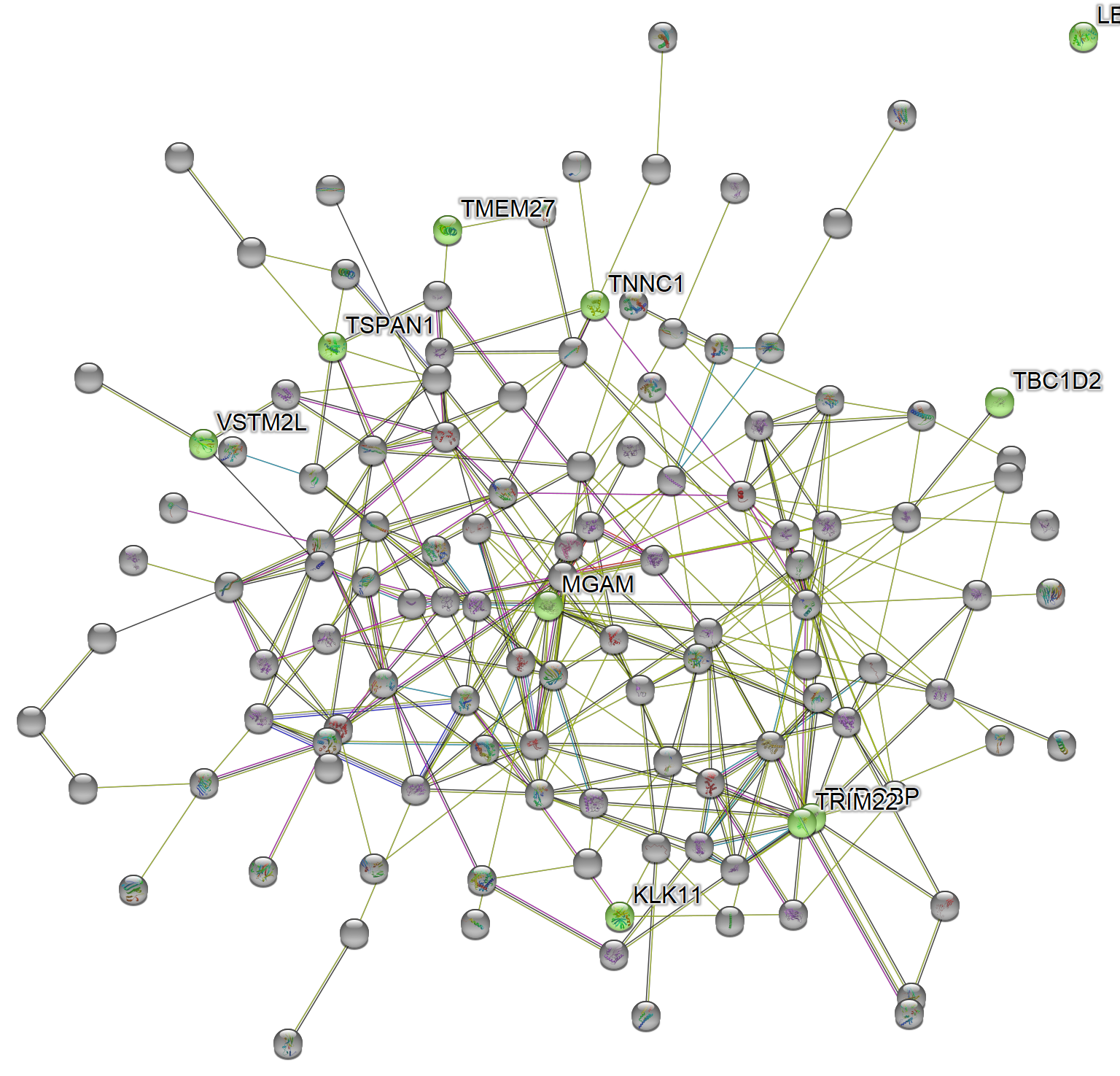
Subnetwork